Sam's X-rays
Assign which regions in image correspond to particles
-
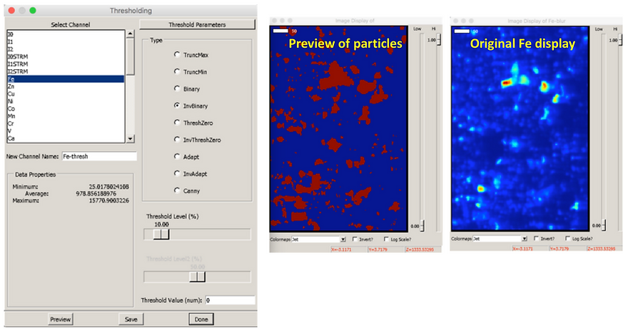
Select “Thresholding” from the “Process” drop down menu. This will bring up the “Thresholding” window where you can make selections….
-
Select the element for which you want to define particles.
-
Select “Inverse Binary": under “type”
-
Select the “Threshold level (%)” by dragging the the scale bar to the desired value, e.g. 10 %. This thresholding method will assign all pixels with an intensity greater than the percentage value selected (e.g. 10 %) to belong to a particle. Any pixels with intensity less than this percentage threshold value will be part of the background and will not be included in your particles.
-
Alternatively, instead of selecting "Inverse Binary" it is also recommended you try "Ostu". This thresholding method selects which pixels comprise particles versus background based on a histogram of intensities in your image.
-
Select “Preview” to see what features are assigned to be particles (the areas shown in red are particles; in blue, background)
-
Compare the preview to the original channel to assess whether your threshold percentage is an appropriate value.
-
If you have a very large range of pixel intensities (e.g. a few very bright spots and many low intensity spots), it may be necessary to set the threshold as low as 2 - 5 %; if you have a small range of pixel intensities (e.g. only low intensity spots), it may be more reasonable to set the threshold to 10 % or so. Use your judgement.
-
Select “Save” to save the calculation as a channel. The name of this channel can be edited in the “New Channel Name” window.
-
Select “Done” to close the window and return to SMAK
Assign minimum number of pixels that make up a particle
-
From the “Analyze” drop down menu, select “Set Minimum Particle Pixels”.
-
A pop up menu will appear. Enter the number of pixels you think are required to constitute a particle. For instance, if you have 3 x 3 micron pixels, but you think that your particles are on the order of 10 x 10 microns, you could set your minimum pixel area to be 3 (9 microns), so that anything smaller does not get counted as a particle. This helps reduce noise.
Compute Particle Statistics
-
Select your threshold channel in the main window of SMAK
-
From the “Analyze” drop down menu, select “Particle Statistics”. A new window will pop up called “Particle Statistics”. This window has four tabs: “Individuals”, “Distributions”, “Box Plots”, and “ANOVA”
Individuals
This window can be used to list the intensity information for each particle, along with particle size and the position of the particle in the image.
Each particle is referred to as a region of interest, or “ROI”. By default, the table shown under the “Individuals” tab will provide a list of all ROI’s identified, the number of pixels comprising that ROI (“Npix”), and the coordinates of the center of the ROI (Xcent, Ycent).
You can convert number of pixels to area by multiplying by the area of an individual pixel.
By highlight an ROI and hitting “Show current”, you can see which particle the ROI corresponds to in your threshold channel. “Show all” will highlight each particle in a different color.
To view the intensity information for an element for each ROI, highlight the element of interest under “Select Channel”. You can choose to view the sum, mean, median or mode of the pixel intensity distribution for each ROI in the table. You can also select whether to view or not view the standard deviation (if mean is selected) in the table. You can highlight multiple channels (either using shift+left click or control+left click) to display their ROI information in the table. After making your selections- WAIT!!! The program is computing this information and it can take a few minutes to finish. Your table will update when the process is complete.
Clicking “Export Data” saves the data to the clipboard and can be directly pasted into an excel spreadsheet.
Currently, clicking “Export Raw Data” does not save the data in a useful format.
Distributions
This tab allows you to view histograms of the ROI size and intensity. You will end up with a plot showing the frequency with which ROI’s of a size or intensity that falls within a certain range of values (or “bin”) occur. For instance, the following plot shows the frequency with which particles containing between 0 and 800 pixels occur. The plot tells you that the majority of the particles are small (containing less than 200 pixels), and there are few particles with sizes between 400 and 800 pixels.
-
Select the element of interest under “Select Channel”.
-
Choose whether you want to see a histogram of the area or the concentration/intensity by toggling the circle next to “Area” or “Conc/Intens”.
-
Select the number of bins, the minimum value for the ROI area/intensity and the maximum value for the ROI area/intensity under “Histogram Options”.
-
If you change your choices you must click “Update”.
-
You can export the plot using “Export”, which saves the plot as a jpeg. Currently, you cannot save the raw data from this plot.
Box Plots
Another way to view the distribution of intensities across all ROIs for each element is using a box plot. The range of intensities is shown for an element of interest for each ROI (the ROI number is displayed on the x-axis) when “ROIs” is toggled below the plot. Also, select the element of interest under “Select Channel”.
On the box plot:
The orange line represents the median
The box represents the upper and lower quartile values
The line represents the range
The crosses represent outliers
If, instead, “Channels” is toggled then the box plot shows the distribution of intensities for a single element for all ROIs, together.
Selecting “Save Graph” will save it as a jpeg (the raw data is not available).
One can assess whether different elements are concentrated in the same ROIs by comparing box plots for the different elements.
ANOVA
The ANOVA tab allows one to examine whether different ROIs exhibit significantly different intensities for a particular element.
-
Select an element under the Select Channels.
-
Highlight the ROIs on which to perform the ANOVA under Select ROI.
-
The ANOVA results will automatically populate in the window. They are color coded such that:
Red text indicates ROIs that are significantly different at the p<0.001 level
Yellow text indicates ROIs that are significantly Green text indicates ROIs that are significantly different at the p<0.005 level
Green text indicates ROIs that are significantly Green text indicates ROIs that are significantly different at the p<0.01 level
Blue text indicates ROIs that are not significantly different (p>0.05)


Thresholding for difficult samples
For some samples it will be particularly difficult to discriminate between overlapping particles. Take the following example, which consists of an Fe(III)-oxidizing biofilm (the string-y objects are bacterial stalks coated in iron oxides):
Clearly, there are many overlapping bacterial stalks forming aggregates, as well as some larger globs of iron. We would like to be able to be able to discriminate between aggregates of bacterial stalks. The following step-by-step process can help.
1. Take the log of the Fe channel in Map Math:
2. Under the "Process" menu in the main SMAK window, select "Advanced Filtering". Then select the LogFe channel and "Mean Shift". Try different filter sizes. This will smooth out gradients in your image:
This will generate a news channel "LogFe-ms", where "ms" stands for mean shift.
3. Under the "Process" menu in the main SMAK window, select "Thresholding", then select your new LogFe-ms channel and select "Otsu" as your thresholding type:
This will generate a new channel, "LogFe-ms-thresh"
4. Go back to the "Advanced Filtering" menu in the main SMAK window and select your new LogFe-ms-thresh channel. Then select "EDT" for Euclidean distance transformation (try different filter sizes). This will try to find the center (red) of the particles versus the edges (light blue), which helps to determine whether a pixel belongs to one particle or another:
This will generate a new channel "LogFe-ms-thresh-EDT".
5. Under the "Analyze"menu in the main SMAK window, choose "Set Watershed Pixel Distance". Lower values tend to work better, but you will need to try different values. In the current example, the default value of 5 was used.
6. Select your LogFe-ms-thresh-EDT, then under the "Analyze" menu, select particle statistics.
Below is a comparison between the particles generated with this method "ms-thresh-edt" versus using ONLY thresholding (either "Otsu" or "InvBinary"). Each particle identified by the thresholding methods is a different color. Although none of the thresholding methods captures the individual bacterial stalks, you can see that the greatest number of particles was identified using the method just described:


